What Is Gini Index In Data Mining

Summary: The Gini Index is calculated by subtracting the sum of the squared probabilities of each class from ane.  It favors larger partitions.  Data Gain multiplies the probability of the class times the log (base of operations=2) of that class probability.  Data Gain favors smaller partitions with many distinct values.  Ultimately, y'all have to experiment with your data and the splitting criterion.

Algo / Split Criterion	Description	Tree Blazon
Gini Dissever / Gini Index	Favors larger partitions. Very simple to implement.	CART
Information Gain / Entropy	Favors partitions that accept small counts but many distinct values.	ID3 / C4.5

We'll talk about 2 splitting criteria in the context of R'southward rpart library.  It's important to experiment with different splitting methods and to analyze your data earlier you commit to i method.  Each splitting algorithm has its own bias which we'll briefly explore.  The code is bachelor on GitHub here.

Using Gini Carve up / Gini Index

• Favors larger partitions.
• Uses squared proportion of classes.
• Perfectly classified, Gini Index would exist zero.
• Evenly distributed would be 1 – (1/# Classes).
• You desire a variable split that has a low Gini Index.
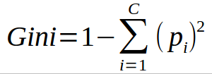
• The algorithm works equally 1 – ( P(class1)^2 + P(class2)^ii + … + P(classN)^2)

The Gini index is used in the classic CART algorithm and is very like shooting fish in a barrel to calculate.

Gini Index:     for each branch in divide:         Calculate percentage branch represents #Used for weighting         for each class in co-operative:             Calculate probability of class in the given branch.             Square the grade probability.         Sum the squared class probabilities.         Decrease the sum from 1. #This is the Ginin Alphabetize for branch     Weight each branch based on the baseline probability.     Sum the weighted gini index for each split.

Here'southward that same process in R every bit a function.  It takes reward of R'south ability to summate sums and probabilities quickly with the prop.table function.  The only departure between the pseudo-lawmaking above and the actual code is that I take into account the Zippo situation where nosotros don't specify a split variable.

gini_process <-function(classes,splitvar = Null){   #Assumes Splitvar is a logical vector   if (is.zippo(splitvar)){     base_prob <-tabular array(classes)/length(classes)     return(1-sum(base_prob**two))   }   base_prob <-table(splitvar)/length(splitvar)   crosstab <- table(classes,splitvar)   crossprob <- prop.table(crosstab,2)   No_Node_Gini <- one-sum(crossprob[,i]**2)   Yes_Node_Gini <- 1-sum(crossprob[,two]**2)   return(sum(base_prob * c(No_Node_Gini,Yes_Node_Gini))) }          

With all of this code, we can apply this on a set of data.

data(iris) gini_process(iris$Species) #0.6667 gini_process(iris$Species,iris$Petal.Length<two.45) #0.3333 gini_process(iris$Species,iris$Petal.Length<five) #0.4086 gini_process(iris$Species,iris$Sepal.Length<6.4) #0.5578          

In this case, we would cull the Petal.Length<two.45 as the optimal variable / condition to divide on.  Information technology has the lowest Gini Alphabetize.

Splitting with Information Proceeds and Entropy

• Favors splits with small counts simply many unique values.
• Weights probability of class by log(base=two) of the form probability
• A smaller value of Entropy is better.  That makes the difference between the parent node's entropy larger.
• Information Gain is the Entropy of the parent node minus the entropy of the kid nodes.
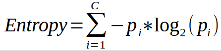
• Entropy is calculated [ P(class1)*log(P(class1),2) + P(class2)*log(P(class2),2) + … + P(classN)*log(P(classN),ii)]

When yous utilise Information Proceeds, which uses Entropy as the base calculation, you accept a wider range of results.  The Gini Index caps at one.  The maximum value for Entropy depends on the number of classes.  Information technology's based on base-2, and then if you lot have…

• Ii classes: Max entropy is i.
• Iv Classes: Max entropy is ii.
• Eight Classes: Max entropy is iii.
• 16 classes: Max entropy is 4.

With that existence said, permit's have a await at how you might calculate Entropy.

Entropy:     for each co-operative in split:         Summate percent branch represents #Used for weighting         for each class in co-operative:             Calculate probability of class in the given branch.             Multiply probability times log(Probability,base=two)             Multiply that product by -1         Sum the calculated probabilities.     Weight each branch based on the baseline probability.     Sum the weighted entropy for each split up.

It's very similar to the Gini Alphabetize adding.  The only real departure is what you do with the course probabilities.  Here information technology is again in R.

info_process <-office(classes,splitvar = NULL){   #Assumes Splitvar is a logical vector   if (is.cypher(splitvar)){     base_prob <-table(classes)/length(classes)     render(-sum(base_prob*log(base_prob,2)))   }   base_prob <-table(splitvar)/length(splitvar)   crosstab <- table(classes,splitvar)   crossprob <- prop.table(crosstab,ii)   No_Col <- crossprob[crossprob[,one]>0,1]   Yes_Col <- crossprob[crossprob[,2]>0,ii]   No_Node_Info <- -sum(No_Col*log(No_Col,2))   Yes_Node_Info <- -sum(Yes_Col*log(Yes_Col,ii))   return(sum(base_prob * c(No_Node_Info,Yes_Node_Info))) }          

Over again, nosotros can run this set of code against our data.

data(iris) info_process(iris$Species) #1.584963 info_process(iris$Species,iris$Petal.Length<two.45) #0.6666667 info_process(iris$Species,iris$Petal.Length<5) #0.952892 info_process(iris$Species,iris$Sepal.Length<6.4) #1.302248          

The difference between the parent Entropy and the Petal.Length of less than ii.45 is the greatest (1.58-0.667) so information technology's still the virtually of import variable.

Data Gain and Gini Alphabetize by Hand

Let's walk through an example of computing a few nodes.

Form	Var1	Var2
A	0	33
A	0	54
A	0	56
A	0	42
A	1	fifty
B	1	55
B	ane	31
B	0	-4
B	1	77
B	0	49

• We're trying to predict the course variable.
• For numeric variables, yous would go from distinct value to distinct value and check the split equally less than and greater than or equal to.

We'll first endeavor using Gini Alphabetize on a couple values.  Let's try Var1 == 1 and Var2 >=32.

Gini Index Case: Var1 == 1

• Baseline of Carve up: Var1 has 4 instances (4/10) where it'due south equal to 1 and 6 instances (half-dozen/x) when information technology's equal to 0.
• For Var1 == 1 & Class == A: 1 / 4 instances have course equal to A.
• For Var1 == 1 & Course == B: 3 / 4 instances have class equal to B.
  • Gini Alphabetize here is 1-((1/4)^2 + (3/four)^2) = 0.375
• For Var1 == 0 & Grade== A: 4 / 6 instances have class equal to A.
• For Var1 == 0 & Course == B: two / 6 instances have grade equal to B.
  • Gini Index here is one-((four/6)^2 + (ii/6)^2) = 0.4444
• We then weight and sum each of the splits based on the baseline / proportion of the data each divide takes up.
  • four/10 * 0.375 + half-dozen/10 * 0.444 = 0.41667

Gini Index Example: Var2 >= 32

• Baseline of Split: Var2 has viii instances (8/10) where it'southward equal >=32 and 2 instances (2/10) when it'south less than 32.
• For Var2 >= 32 & Grade == A: five / eight instances have course equal to A.
• For Var2 >= 32 & Class == B: three / viii instances take course equal to B.
  • Gini Index here is i-((5/8)^2 + (3/8)^ii) = 0.46875
• For Var2 < 32 & Grade == A: 0 / ii instances have class equal to A.
• For Var2 < 32 & Class == B: 2 / 2 instances have class equal to B.
  • Gini Index hither is 1-((0/2)^2 + (2/2)^two) = 0
• Nosotros and so weight and sum each of the splits based on the baseline / proportion of the data each split takes upwards.
  • 8/10 * 0.46875 + two/10 * 0 =0.375

Based on these results, you would choose Var2>=32 as the separate since its weighted Gini Index is smallest.  The adjacent step would be to have the results from the split and further division.  Allow'southward take the 8 / 10 records and try working with an Information Proceeds Dissever.

Class	Var1	Var2
A	0	33
A	0	54
A	0	56
A	0	42
A	1	l
B	1	55
B	one	77
B	0	49

Information Gain Example: Var2<45.5

Again, we'll follow a similar procedure.

• Baseline of Divide: Var2 has 2 instances (two/8) where it's < 45.5 and 6 instances (vi/eight) when it'south >=45.v.
• For Var2 < 45.five & Class == A: two / 2 instances have course equal to A.
• For Var2 < 45.v & Class == B: 0 / 2 instances take form equal to B.
  • Entropy here is -1 * ((ii/2)*log(2/2, ii)) = 0
  • Notice how class B isn't represented here at all.
• For Var2 >= 45.5 & Form == A: 3 / 6 instances have grade equal to A.
• For Var2 >= 45.5 & Class == B: three / 6 instances have class equal to B.
  • Entropy hither is -one * ((3/6)*log(three/6, ii) +(three/6)*log(three/6, two)) = 1
• We and so weight and sum each of the splits based on the baseline / proportion of the data each separate takes up.
  • 2/8 * 0 + 6/8 * one =0.75

Information Gain Example: Var2<65.5

• Baseline of Split: Var2 has vii instances (7/viii) where it's < 65.5 and 1 instance (1/8) when it's >=65.5.
• For Var2 < 65.v & Class == A: 5 / vii instances accept class equal to A.
• For Var2 < 65.five & Grade == B: ii / 7 instances take form equal to B.
  • Entropy hither is -1 * ((5/7)*log(five/7, ii) +(2/seven)*log(two/7, 2)) = 0.8631
• For Var2 >= 65.five & Class == A: 0 / 1 instances have grade equal to A.
• For Var2 >= 65.5 & Grade == B: 1 / ane instances have form equal to B.
  • Entropy here is -1 * ((1/i)*log(1/1, 2)) = 0
  • Notice how class A isn't represented hither at all.
• We then weight and sum each of the splits based on the baseline / proportion of the data each split takes up.
  • vii/8 * 0.8631 + 1/eight * 0 =0.7552

Based on Information Gain, we would choose the split that has the lower amount of entropy (since it would maximize thegain in information).  Nosotros would choose Var2 < 45.5 as the side by side split to use in the determination tree.

As an exercise for you, try computing the Gini Index for these two variables.  Yous should see that we would choose Var2 < 65.5!

When Information Gain and Gini Index Choose Unlike Variables

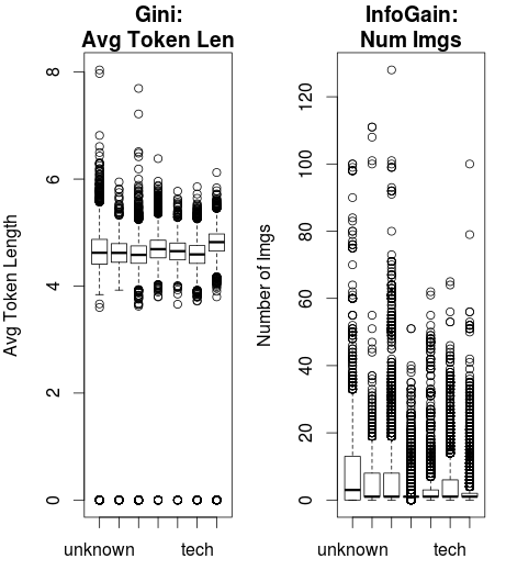
The differences are much more intuitive when yous await at some real information and how the splitting method would make an impact.

This information from the UCI Machine Learning Repository shows the popularity of webpages from Mashable.  Two variables, Average Token Length and Number of Images are entered into a classification conclusion tree.

Using Gini Index equally the splitting criteria, Average Token Length is the root node.

Using Information Gain, Number of Images is selected as the root node.

You can run into the relatively tighter spread of the Boilerplate Token Length and the wider dispersion of the Number of Images.

Ultimately, the choice you brand comes down to examining your data and being aware of the biases of your algorithms.  Again, the code for this example is available on GitHub here.

What Is Gini Index In Data Mining,

Source: https://www.learnbymarketing.com/481/decision-tree-flavors-gini-info-gain/

Posted by: nelsonhisguallon.blogspot.com

Share this post